Fig.1 - Illustration of the reflection (specular here) of light
at an interface.
Last update, Sept. 9, 1998
Institute for Computer Graphics, Graz University of Technology,
Muenzgrabenstr. 11, A-8010 Graz, Austria
and
LEMS, Brown University, Providence, RI 02912, USA
Sept. 1998 - DRAFT
Abstract
1 - Introduction
2 - A new computational paradigm for
light rendering in graphics
3 - Wave propagation in Geometrical
Optics : Cellular automata & Distance Transforms
4 - Computational Challenges
References
Form factor evaluation for free form surfaces and General Visibility computations for realistic rendering tasks, through radiosity or multiple reflectance/transmission ray tracing, remain open problems in Computer Graphics. We propose a new paradigm, based on a physically-based simulation of wave propagation in 3D media, to disentangle this apparent bottleneck between the needs for accuracy and realtime interactions. Our method is based on an off-line processing of a General Visibility Data Structure, through the recently developed concept of CADT: Cellular Automata based on (Euclidean) Distance Transforms.
Consider a static 3D modeled scene made of various objects, say buildings, cars, street-lights, etc., for an outdoor view, and furniture, lamps, books, glasses, rugs, etc., for an indoor set. The general rendering problem involves massive calculations to evaluate light interactions between the different surface patches of these objects. Two principal methods have been studied in the Graphics community to perform rendering of a 3D scene and produce realistic images, namely radiosity and ray tracing. In radiosity computations one aims at evaluating the - diffuse - exchange of energy between the surfaces of the scene, a view-independent calculation. In ray tracing, one computes specular reflections and transmission of light in a view-dependent calculation.
A radiosity computation, for a given scene, is one which, starting from an assumption of energy equilibrium, calculates (approximately) how much energy is being reflected from any given surface, due to all other surfaces interchanging energy with it. This allows for soft lighting effects, colour bleeding from one surface to another and non point-source lighting.
In ray tracing, a ray of light is traced in a backward direction. That is, we start from the eye or camera and trace the ray through a pixel in the image plane into the scene and determine what it hits, how it is reflected and/or transmitted, this possibly a multiple number of time. The pixel is then set to the color values returned by the ray. Ray tracing is good at providing sharp edges and mirror-like reflection effects, something radiosity can hardly do.
Radiosity is usually computed off-line, with or without light-sources, as it is view-independent in nature. One then combines its result with a view-dependent rendering process, generally a ray tracing stage, to compute the final image for a particular view (eye position). A full ray tracing rendering is view-dependent of course.
Some attempts have been made at combining the two methods to benefit from their respective advantages [Sillion89]. Still, such approaches fall into the paradigm of polyhedral worlds.
We propose a shift of paradigm for rendering. We wish to incorporate advantages of both the well-established techniques described above, while allowing to tackle the General Rendering problem outlined above, where realistic natural objects can take convoluted forms and are not limited to polyhedral or triangulated surface representations, as is usually the case in the large majority of renderer available today.
In particular, we aim at rendering realistic scenes such that:
In the following paragraphs, we outline the proposed new paradigm for light rendering.
In its classical formulation light can bounce off a surface or be transmitted through it, or both. This change of light direction at an interface can be a function of wavelength, time, and orientation.
Whether we approximate or not the physics involved in modeling the interaction of light at an interface, we are bound in all approaches to compute the visibility function at a surface (point or patch). The visibility function tells you what can be seen in a sphere of direction around a point. If only reflectance is considered, this sphere reduces to an hemi-sphere, see Fig.1, at most points. That is, we can locally approximate the neighborhood of a surface point to be flat or part of a small plane - in differential geometry, this is a first order approximation by a tangent plane, always valid at smooth points.
Fig.1 - Illustration of the reflection (specular here) of light
at an interface.
Essentially, rendering systems need to have access to visibility information to know which part of light energy will be captured by other surfaces, and which part will be lost (e.g. in the sky).
Any algorithms which computes light interaction at interfaces, with main goal to render the scene where light is propagated, need in one form or another such visibility information.
In the case of polyhedral objects, recent results demonstrate the usefulness of computing some representation of the full visibility information for a given static scene [Drettakis97 , Durand97 , Elber98].
Visibility becomes an "intrinsic property of geometric models", similarly to texture, color, proximity, etc. [Elber98]. In essence, a Global Visibility Data Structure can be used to speed-up some of the most demanding computational process in rendering, namely form factor evaluation, ray casting, shadowing, etc.
In order to compute visibility in a general setting, i.e., without assuming particular geometries of the shape of objects, such as the traditional polygonal/hedral representation, we can simulate light transport as a physical process.
Still, many physical models are available, depending on the type of phenomena one wishes to model: optical, radar, quantum physics, ...
For Computer Graphics applications, it is useful and sufficient in most practical cases, to consider only the so-called geometrical optics model.
In essence, in the general wave equation describing the physics of light propagation, we do not consider wavelength effects. Then, the wave equation reduces to the so-called eikonal equation:
|| Nabla{ S }|| = µ
In this context, the wavefront time arrival S is only a function of the metric properties of the medium (3D space optical characteristics). In most cases, we can assume the refractive index to be constant and equal to unity. Then, light propagation is equivalent to the so-called Euclidean Distance Transform (EDT), which maps, for any source point of propagation, the surrounding space with distance values from this source [Leymarie92].
We thus propose to replace the computation of visibility in Graphics rendering problem, by the equivalent problem of computing a distance transform of the 3D intermediary (with respect to objects) space, for sources taken on the surface of objects. These "sources" are the loci where visibility is required to be known.
The model for visibility computation we propose to explore shall permit us to:
Let Phi(q0, t) be the wavefront of the point q0 after time t. For every point q of this front, consider the wavefront after time s: Phi(q, s).
Then, the wavefront of the point q0 after time s+t, Phi(q0, s+t), will be the envelope of the fronts Phi(q,s), such that q in Phi(q0,t).
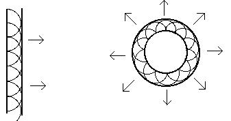
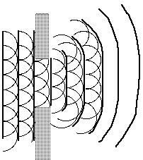
Fig.2 Illustration of Huygens' principle.
In this formulation, one can replace the "point" q0 by a curve, surface, or in general, by a closed set. Furthermore, the 3D space can be replaced by any smooth manifold, and the propagation of light can be replaced by the propagation of any disturbance transmitting itself "locally" [Arnold89].
We can also replace the metric from Euclidean to a Riemannian, and model anisotropic "shape" properties (of the "participating" medium, or space).
The difficulty, is to translate this principle in a discrete world relying upon a lattice, such as the X-Y-Z grid made of voxels, traditionally used in image processing.
We have developed such a "discrete" method relying upon a 3D grid. We call it 3D-CADT for:
In this approach, we simulate propagation of information by the use of a class of cellular automata "oriented" in the direction of the wavefront. Equivalently, these automata rely upon the metric characteristic of the underlying space (the "indicatrix"). For Euclidean 3D space, this is a sphere of directions.
In the context of symmetry elicitation, for example in the computation of light caustics, rather than let cellular automata propagate independently, to compute the visibility of each source, we propagate them together: i.e., each photon (or cellular automaton) is restricted in its propagation by neighboring photons (this is one way of understanding Huygens' principle), thus propagating along a ray.
The resultant ray system, is the system of "normals" to a surface in Euclidean space. In the neighborhood of a smooth surface, its normals form a smooth fibration, until at some distance from the surface, various normals may begin to intersect one another.
Historical note: These "singularities" were first investigated by Archimedes (caustics of light rays, around 300 B.C.).
Fig.3 Initial level sets (d=3) from a sphere and a plane
together with
resultant medial axis (a parabola).
Fig.4 Initial level sets (d=10) from a sphere and a plane
together with
resultant medial axis (a parabola).
In essence, what I imagine is computing off-line the visibility (hemi-)sphere for all surface "points" of the (static) objects in the scene.
Let us consider the case of a single point. (A "point" might become a "patch" for planar elements.) Using my method of 3D wave propagation I can compute the full visibility function for that point. The result is that I can segment and label the sphere of directions for the source point in terms of visible object points/patches (those which are reached by the wavefront).
The visibility function for a given surface point is "full" or complete, because we simulate accurately the eikonal equation and are able to fill-in space with perfectly straight rays at sub-voxel accuracy, i.e. in a continuous manner. The reason for the latter, is the use of the Euclidean metric, rather than some approximation. Furthermore, we minimize the computational load, by our clever (!) design of cellular automata, mimicking the behavior of photons.
What is the expected numerical load then? Suppose our "space" is a cube of size N voxels. suppose we have M "points" to represent our scene geometry in this cubic space. Then for any given surface point, the complexity of the visibility computation has a max bound of 4xN. In fact, this is a bound for the case where the point is isolated in space (a spherical wavefront fills space). The "4" comes from (some of) the "masks" used to propagate information (hint: that "4" becomes a "2" in 2D). Equivalently, each cellular automaton (photon) may generate at most 3 more cellular automata when propagating, in order to fill the (discrete) space with light rays.
Thus, the more complex the geometry of the scene, the lower the expected numerical load for each point (in other words, the more "crowded" the scene is when viewed from any surface point, the lesser the portion of space that will be visited by the associated light wave). On the other hand, of course, the more points are needed to describe geometry, the more times I have to compute visibility (although this is certainly not linear ... neighbors on the surface can benefit from the nearby computed visibility).
Let us suppose for now that for each surface point the numerical load is much lower than 4N; let us replace 4 by a factor "a" (a << 4). Then, a maximal bound on complexity for visibility computation would be tantamount to aNM. Note that here N is fixed, M varies as a function of shape or object complexity and a equals some unknown function of M (well we know it is inversely proportional to M, not necessarily in a linear fashion). Also, we should really restrict N to some bounding box around the shape in the cubic space (visibility to infinity is not used here).
At first approximation, the numerical load for accurate visibility computation for freeform shapes seems quite tractable. Furthermore, this visibility computation is computed off-line for a given scene and it can be parallelized: we consider each source as independent and we propagate a light wave in the medium surrounding objects, to retrieve its own visibility sphere.
The principal difficulty seems to lie in the representation of "visibility" once computed. For each point we now know which other points occlude our view in the sphere of direction around us. In practice, the sphere becomes an hemi-sphere for most points. We now have to discretize this hemisphere in terms of spherical or solid angles somehow. Well in fact, we only need to store in a look-up table the "other points" (labels) that were encountered during propagation, together with the angles (locus) they represent in our "sky" (a function of 2 parameters say).
Therefore, a brute force solution could be to store in a look-up table, for each surface point, the labels of other surface points directly visible in its visibility sphere. This assumes each object surface points has been given a label (a number) a priori. The look-up table would be discretized in bins, where the visibility sphere is quantized as a function of 2 solid angles.
In each such bin a varying number of labels can be stored. With each label, we could further associate the precise angle values of visibility, the distance a ray has to travel to reach the "visible" point, etc. But in fact, this is not necessary, especially if our memory resources are limited and if exact computations are required: since we have a label of an object surface point, we can retrieve the necessary information to obtain the desired values, by accessing on-line the surface points' properties, e.g. its 3D coordinates (this is a typical trade-off between memory and realtime constraints).
The fineness of the grid used to quantized the visibility hemisphere should be variable and maybe even adaptable. There should probably be more (smaller) bins right above the surface point (in the surface normal direction). This variable sampling may be adapted due to the local geometry of the object. For example, along a ridge, the previous comment is not necessarily accurate, while it is at the bottom of a valley.
An interesting byproduct of this representation of the "sky" for each surface point is that we can naturally introduce the effect of having "real" empirical BRDFs - like the one Mark Levoy (Stanford Graphics Lab.) will sample in Italy, or the one we already sampled in the REALISE project [Leymarie96] - to modulate paths reflectance when we will compute full paths in Metropolis-like rendering (i.e. by propagating multiple-reflection paths with a certain stochastic process) [Veach97 ].
Consider using the Metropolis light transport algorithm for light rendering. We now introduce light sources and an eye (or eyes ...). We can start propagating from the eye the stochastic paths (random walks in 3D space) to compute a kind of probabilistic visibility of this eye, its "sky". Similarly for the light sources (seen as points or sets of points). The new result here is that we now have accessible the full set of pencils of light paths of use to render our scene. The Metropolis can be used to more efficiently render a complex scene. Furthermore, if we modify eye pose or light pose, we mainly have to recalculate a cone of visibility for the eye or light only... the scene remaining static after all.
What is the complexity of this eye and light visibility computation? Something like (b+c)N where b and c depend on M, but are expected to be a very small fraction of 4.
If in Metropolis transport, the visibility computation is a problem (tantamount to ray casting it seems), then the above seems a good approach. We have not computed full optical paths, but only sub-paths (visibility pencils). We now have to connect these through look-up table and as a function of material properties and the stochastic ray shooting sampler.
Nevertheless, even if our method would not provide such of a gain over "traditional" methods of computing visibility, note that it permits to use freeform surface representations, and implicitly allows for the use of real BRDFs (or even the BSDFs).
Furthermore, our approach seems amenable to render scenery with participating media (smoke, clouds, ..., aquariums, lens, etc.).
Also, if the scenery is locally modified, deformed, it should be relatively easy to update only the right (perturbed) visibility skies ... without recomputing the other pencils, this because we simulate light wave propagation.
And finally, note that we have a direct way of retrieving caustics, that is those loci where light rays intersect (on a surface or in space, if there is some dust in the air for example).
In summary, we have traded on line path-computation for memory space (to store the "skies"). Is it worth it? it ought to be.
© Frederic Leymarie,
1998.
Comments, suggestions, etc., mail to: leymarie@lems.brown.edu